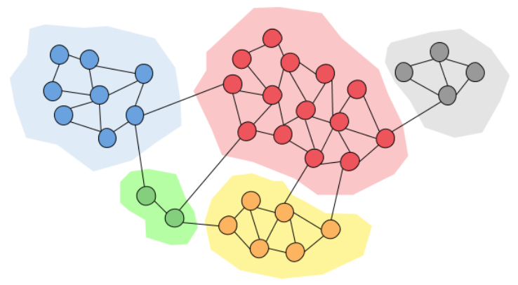
Community detection is the problem of finding communities: sets of densely connected nodes within a graph. Think of it as a form of clustering. Methods like GraphRAG use exactly this technique to break a knowledge graph into manageable pieces. This post covers where modularity, the most widely used metric in community detection, comes from. It then compares Louvain and Leiden, the two algorithms most commonly used to optimize it.
Modularity: Measuring How Well-Formed a Community Is
Say you’ve formed a community. What does it mean for that community to be “good”? The most common answer in community detection is a metric called modularity. The intuition is simple: compute how many edges you’d expect inside this community if the graph’s edges were wired up completely at random, then measure how far the observed edge count exceeds that expectation. If the connections are too dense to explain away as coincidence, that’s evidence you’ve found a real community.
For the simplest case, just two communities, modularity is defined as:
$$ Q = \frac{1}{2m} \sum_{vw} \left[A_{vw} - \frac{k_v k_w}{2m}\right] \frac{s_v s_w + 1}{2} $$Let’s unpack the notation. $Q$ is the modularity value itself, and $m$ is the total number of edges in the graph. $A_{vw}$ is the adjacency matrix: 1 if nodes $v$ and $w$ are connected, 0 otherwise. $k_v$ is the degree of node $v$, the number of edges attached to it.
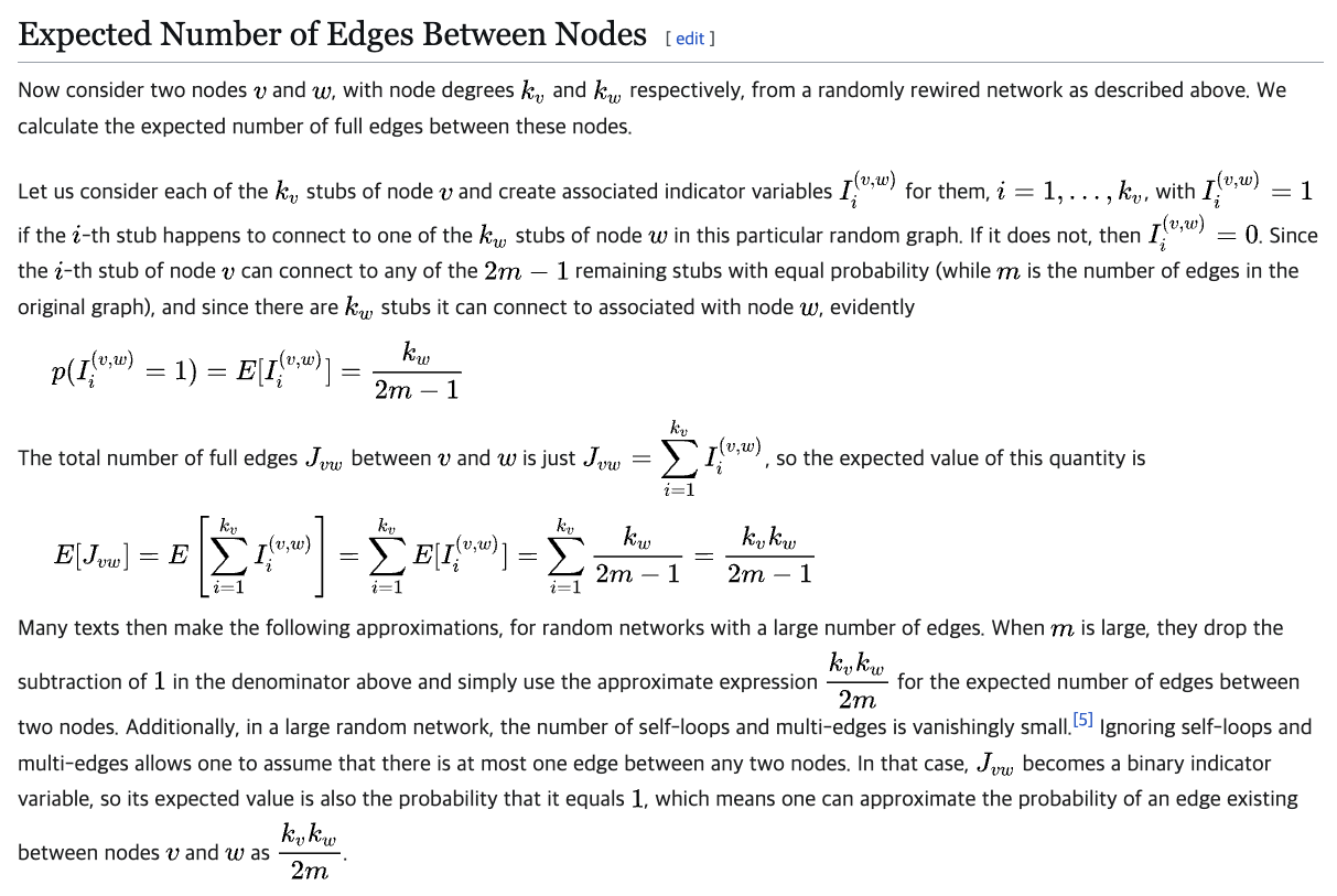
The key term is $\frac{k_v k_w}{2m}$. This is the null model, the probability that an edge exists between $v$ and $w$ if the graph’s connections were shuffled completely at random. It accounts for the fact that even under random wiring, a higher-degree node is more likely to end up connected to any given node. So $A_{vw} - \frac{k_v k_w}{2m}$ is the observed connection minus the connection you’d expect by chance, in other words, how far the connection between $v$ and $w$ exceeds what pure coincidence would explain.
The term multiplying it, $\frac{s_v s_w + 1}{2}$, is spin-variable notation borrowed from physics, constructed so it equals 1 if $v$ and $w$ are in the same community and 0 otherwise. So modularity sums up that “excess over chance” term, but only over node pairs that share a community.
The sign of $Q$ is meaningful on its own. $Q > 0$ means the community’s internal connections are denser than random chance would produce, so it’s not coincidental. $Q = 0$ means the community looks no different from random. $Q < 0$ means the connections are sparser than random.
Multiple Communities: The Generalized Form
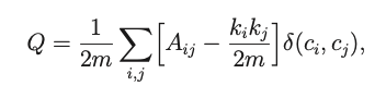
The formula above assumes exactly two communities. Generalize it to an arbitrary number of communities and the spin-variable term becomes a Kronecker delta:
$$ Q = \frac{1}{2m} \sum_{vw} \left[A_{vw} - \frac{k_v k_w}{2m}\right] \delta(c_v, c_w) $$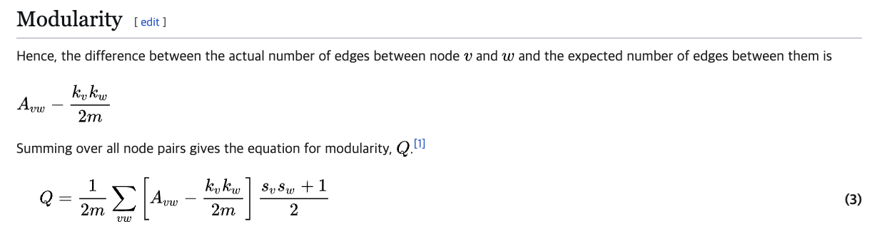
Here, $\delta(c_v, c_w)$ returns 1 if $v$ and $w$ belong to the same community and 0 otherwise, generalizing the earlier spin-variable term to work regardless of how many communities exist. Everything else about the formula, and how to read it, stays the same.
Resolution: A Dial on What Counts as “Random”
You can add one more parameter here: resolution, $\gamma$.
$$ Q = \frac{1}{2m} \sum_{vw} \left[A_{vw} - \gamma \frac{k_v k_w}{2m}\right] \delta(c_v, c_w) $$Notice $\gamma$ multiplies the null-model term, $\frac{k_v k_w}{2m}$. Shrink it, and the baseline for “how connected this would be by chance” drops. A lower baseline makes it easier for a new node to increase modularity when added to a community, which lets even relatively weakly connected nodes join the same community. Turning $\gamma$ down pushes the result toward fewer, larger communities.
The Louvain Algorithm
Louvain, proposed in 2008, is the standard algorithm for optimizing modularity. It alternates between two phases. Local Moving examines each node in turn and greedily assigns it to whichever neighboring community would increase overall modularity the most. Once Local Moving stops finding improvements, Aggregation collapses every community found so far into a single node, producing a new, smaller graph. Local Moving then runs again on that collapsed graph, and the two phases keep alternating.
The algorithm stops under any of three conditions: Local Moving no longer moves any node, overall modularity stops increasing, or Aggregation no longer shrinks the graph. The output is a hierarchical community structure, along with which community each node belongs to at each level.
The Leiden Algorithm: Patching Louvain’s Gap
Louvain has a weakness. Because it optimizes purely for overall modularity, it can produce disconnected communities, groups where nodes get labeled as belonging together even though no path connects them internally. This can happen depending on the order in which Local Moving visits the nodes, leaving a community with disconnected parts.
The Leiden algorithm targets exactly this problem. It’s designed to guarantee that every node inside a community can reach every other node in it. It does this by inserting a new phase, Refinement, between Louvain’s two existing phases. After Local Moving finds communities, Refinement temporarily resets every node inside each community back to its own individual community. From there, only nodes that are well-connected to each other get merged back together; disconnected nodes stay on their own. Only after this refinement does the algorithm move on to Aggregation. By cycling through Local Moving, Refinement, and Aggregation, Leiden produces communities that are internally connected, at roughly the same computational cost as Louvain.