Background
Frequent HBM Access Creates an I/O Bottleneck in Standard Attention
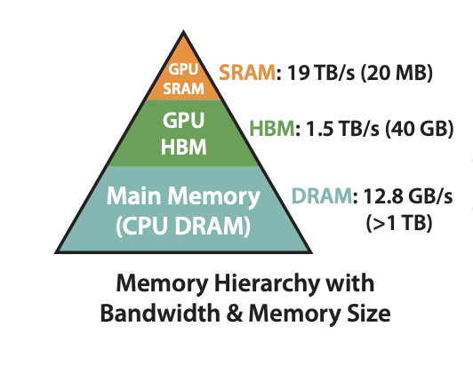
The authors focus on the I/O bottleneck in attention, pointing to the frequent HBM accesses in standard implementations as a major cause. To understand what is going on, we first need to look at the memory hierarchy found in GPUs and most other accelerators.
Improving Actual Wall-Clock Time, Not Just Reducing FLOPs
The authors note that previous work has tried to reduce the compute and memory complexity of attention, but many of those studies do not report improvements in actual wall-clock time. Their explanation is that these approaches tend to focus on reducing theoretical operation counts while overlooking the overhead of memory access.
To make attention faster in practice, they argue, we need to pay attention to this memory bottleneck. This is really the central argument of the paper. They propose FlashAttention, an IO-aware redesign of attention that reduces data transfers between SRAM and HBM.
The Memory Hierarchy
For this discussion, we can think of GPU memory in terms of on-chip SRAM and HBM, which serves as the GPU’s main memory. The fast SRAM available to each SM (streaming multiprocessor) has very high bandwidth but very little capacity. HBM has much more room, but its bandwidth is considerably lower. To draw a rough analogy with the more familiar CPU, SRAM plays a role similar to on-chip cache memory, while HBM is closer to the DRAM connected to the CPU. The analogy is about speed and capacity, rather than identical memory-management behavior.
(Note to self: check whether comparing an SM to a CPU core is a useful analogy.)
The Dilemma in Attention Computation
The trade-off in this paper is one that comes up all the time in computing. SRAM is fast but small; HBM is large but slower. Put simply, fewer accesses to slow HBM mean less I/O overhead. But SRAM is too small to hold all the intermediate results of standard attention, so those results end up being stored temporarily in HBM.
How Attention Is Computed
To tackle this dilemma, the authors take a closer look at how attention is actually computed. For an input sequence of length $N$, the attention output $O$ is calculated from its query, key, and value representations. The important detail here is that the intermediate matrices $S$ and $P$ each have shape $(N, N)$: their size grows quadratically with the sequence length. The paper identifies the I/O overhead of reading and writing these large matrices as a major reason attention is slow.
Let’s walk through the standard computation step by step to see where that overhead comes from.
- Read blocks of $Q$ and $K$ from HBM into SRAM, compute $S = QK^T$, and store the result in HBM.
- Read $S$ back from HBM, apply softmax row by row to compute $P = \operatorname{softmax}(S)$, and store the result in HBM again.
- Read blocks of $P$ and $V$ from HBM, compute the final attention output $O = PV$, and write $O$ to HBM.

Including the usual scaling factor, the equations for a single attention head are:
$$ S = \frac{QK^{\mathsf{T}}}{\sqrt{d}}, \qquad P = \operatorname{softmax}_{\mathrm{row}}(S), \qquad O = PV $$$$ Q, K, V, O \in \mathbb{R}^{N \times d}, \qquad S, P \in \mathbb{R}^{N \times N} $$As in Algorithm 1, I will omit the scaling factor in the walkthrough below.

In this process, we write the score matrix $S$ to HBM and then read it back for softmax. We also write the resulting weight matrix $P$ to HBM, only to read it back when computing the final output. Since both matrices have shape $N \times N$, this memory I/O becomes more expensive as the input grows. Could we use the intermediate results directly in the next operation, without storing them in HBM? At this point, we can start to see where the paper is heading.
Let’s find a way to compute the exact attention output $O$ without copying the huge intermediate matrices $S$ and $P$ to HBM!
Now that we have the motivation, let’s look more closely at how the paper computes the exact output without moving those entire intermediate matrices to HBM.
FlashAttention
The goal is clear.
Given $Q$, $K$, and $V$, compute the exact attention output $O$ while minimizing HBM access!
The central idea is to split $Q$, $K$, and $V$ into blocks and accumulate the attention output block by block, eliminating the need to store the full intermediate matrices $S$ and $P$ in HBM.
Tiling
To compute the intermediate weight matrix $P$, we need to apply softmax to the score matrix $S$.
$$ P = \operatorname{softmax}(S) $$The paper divides $Q$, $K$, and $V$ into blocks and computes their contributions to the output $O$ one block at a time. The aim is to eliminate the memory I/O involved in storing the intermediate matrices $S$ and $P$ in HBM.
There is a problem, though. Applying softmax independently to each block does not give the same result as applying it to the entire row. Softmax exponentiates each element of a vector and divides it by the sum of all the exponentials. For finite inputs, the resulting values are positive and sum to 1, forming a probability distribution. In practice, the paper subtracts the maximum before exponentiating to prevent overflow.
$$ \operatorname{softmax}(x)_i = \frac{e^{x_i}}{\sum_{j=1}^{n} e^{x_j}} $$
To compute softmax correctly, we need the sum of the exponentials across the entire vector. Yet the paper computes blockwise quantities and uses correction factors to recover the normalization for the full vector. How can a calculation based on partial sums give the same result as normalization by the full sum? Let’s look a little deeper.
The key is to use a basic property of exponentials to rescale the blockwise results.

Multiplying exponentials is equivalent to adding their exponents.
$$ e^{a+b} = e^a \cdot e^b $$With this identity in mind, the following equation becomes fairly straightforward.
By multiplying a blockwise result by the appropriate correction factor, we can express it relative to the maximum of the full vector.
$$ \underbrace{e^{x_i^{(1)}-m(x)}}_{\text{Full-vector reference}} = \underbrace{e^{x_i^{(1)}-m(x^{(1)})}}_{\text{Block reference}} \cdot \underbrace{e^{m(x^{(1)})-m(x)}}_{\text{Correction factor}} $$To keep track of the rescaling and normalization, the algorithm stores the running maximum $m$ and exponential sum $\ell$ separately.
Algorithm
Here is the core algorithm from the paper.
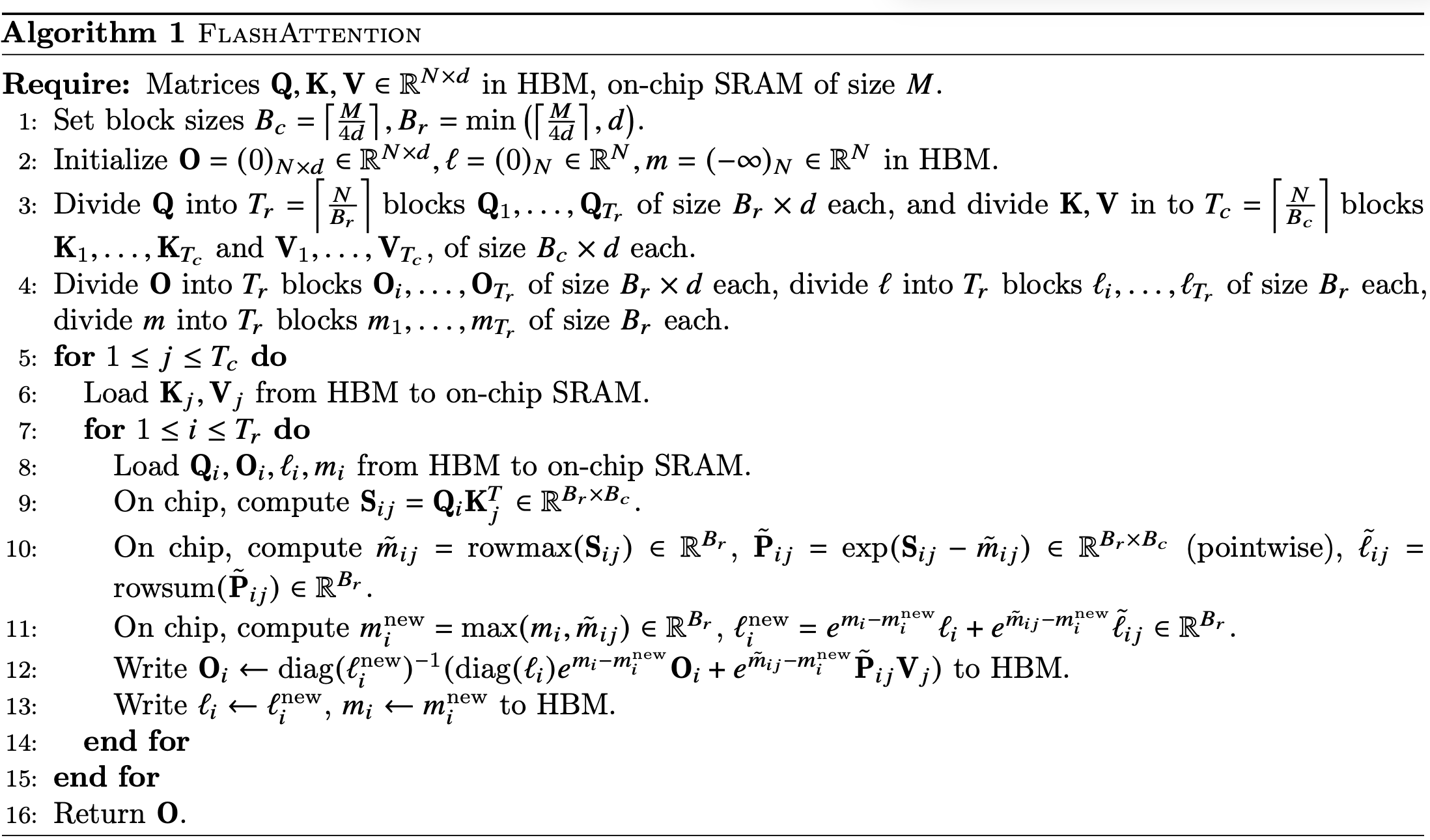
Let’s go through it one line at a time.
Line 1

This step chooses block sizes so that the data needed to process a tile can fit in SRAM. Appendix C, in the proof of Theorem 2, discusses the space requirements in more detail.
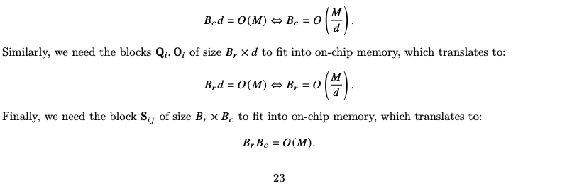

We can roughly account for the data needed to process one tile as follows:
- $K_j$ and $V_j$: each has shape $B_c \times d$.
- $Q_i$ and $O_i$: each has shape $B_r \times d$.
- $S_{ij}$: has shape $B_r \times B_c$.
As the head dimension $d$, tile height $B_r$, or tile width $B_c$ increases, processing a tile requires more memory. But the working data still has to fit in the available SRAM. In other words, these dimensions are constrained by the SRAM capacity $M$. Since the head dimension and available SRAM are generally fixed for a given model and device, we need to choose the tile dimensions accordingly. The column block size therefore scales with $M/d$, while the row block size also has the paper’s additional upper bound of $d$. Here, $T_r$ and $T_c$ denote the number of blocks, rather than the dimensions of a block.
I could not find a separate derivation for the constant $4$. In an actual implementation, it seems that we would also need to account for details such as the data types of $Q$, $K$, and $V$ (FP32, for example) when choosing appropriate block sizes.
Line 2

Next, we allocate space for the accumulated results. First comes an $N \times d$ matrix for the attention output $O$. We also allocate the length-$N$ vectors $\ell$ and $m$, which hold the per-row statistics needed to rescale the blockwise contributions.
Lines 3–4

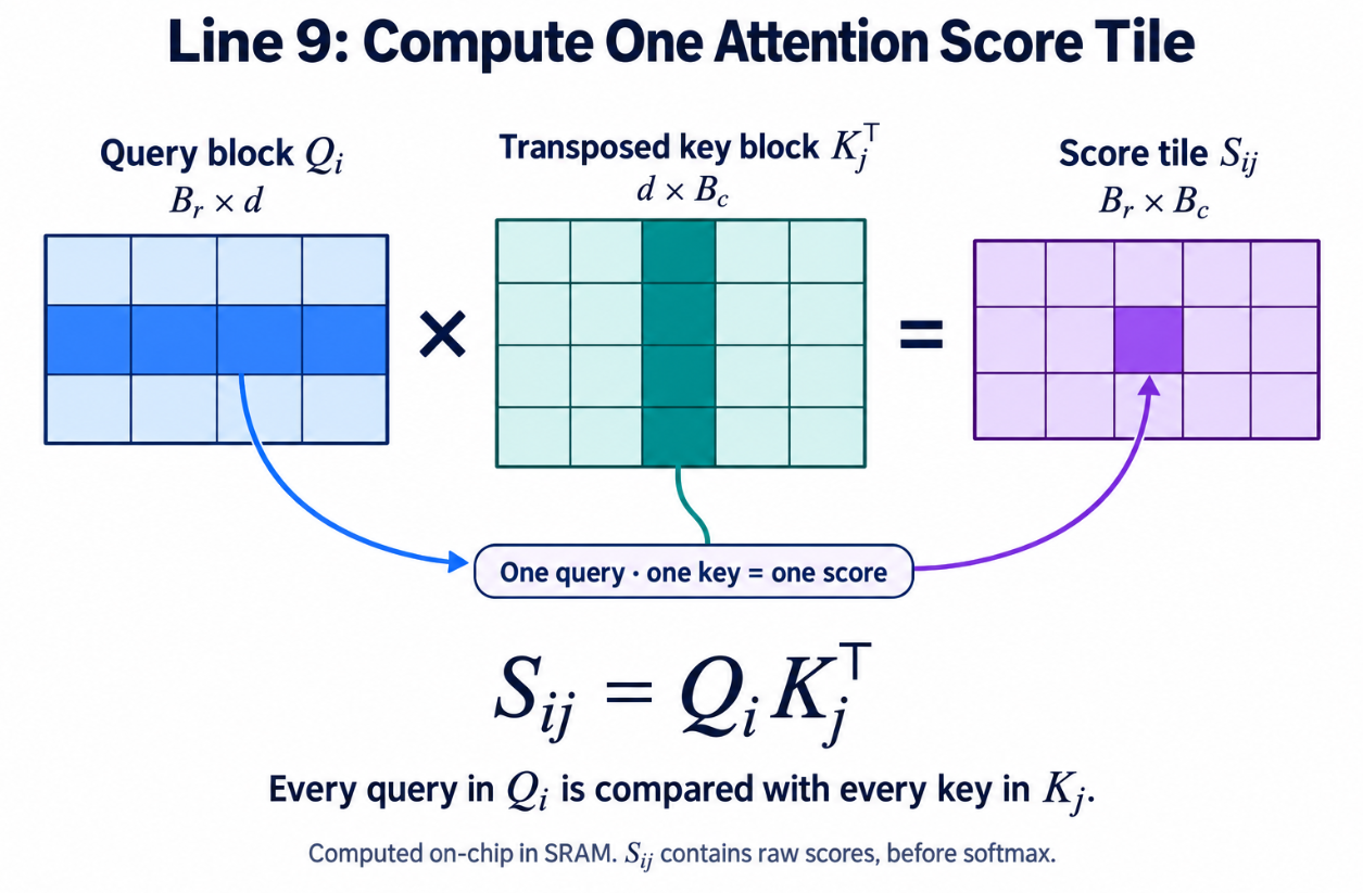
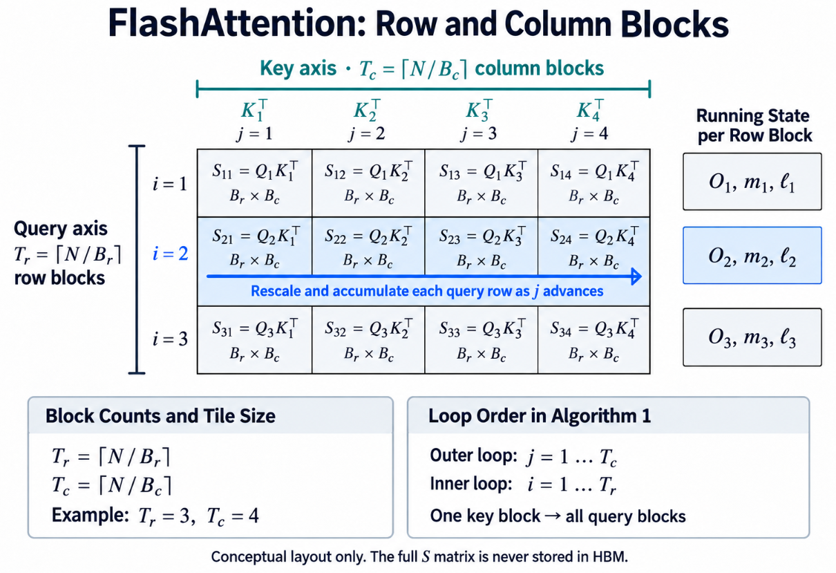
Now we divide the matrices into blocks. The query matrix $Q$ is split into $T_r$ blocks of shape $B_r \times d$, taking $B_r$ rows at a time. The key and value matrices $K$ and $V$ are each split into $T_c$ blocks of shape $B_c \times d$. The score tile $S_{ij}$ therefore has shape $B_r \times B_c$.
The output $O$ and the statistics $\ell$ and $m$ are partitioned along the same query rows. Each $O_i$ is a $B_r \times d$ matrix, while $\ell_i$ and $m_i$ are length-$B_r$ vectors.

Lines 5–6
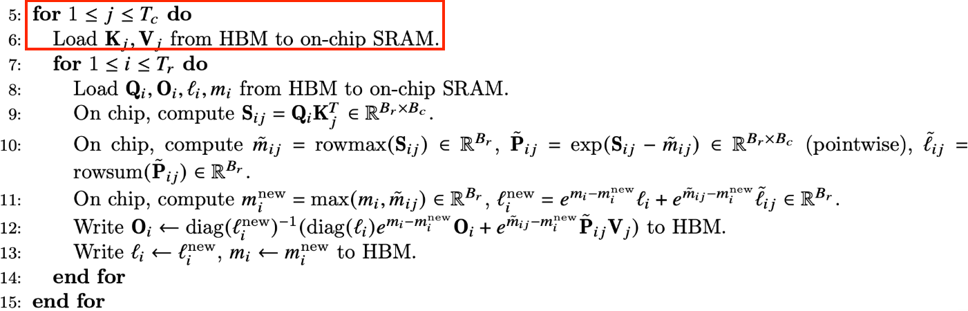
To compute all the outputs, we need to visit every combination of the $T_r$ row blocks and $T_c$ column blocks.
The algorithm uses two nested loops. In terms of the score matrix $S$, it works through one column block at a time, with the outer loop running from $1$ to $T_c$. Lines 5–6 begin this outer loop and load the key and value blocks $K_j$ and $V_j$.
An interesting detail is that this loop order changes in the follow-up paper, FlashAttention-2, where the forward algorithm places query blocks in the outer loop. I will leave a closer look at that decision for a review of the next paper.
Lines 7–9
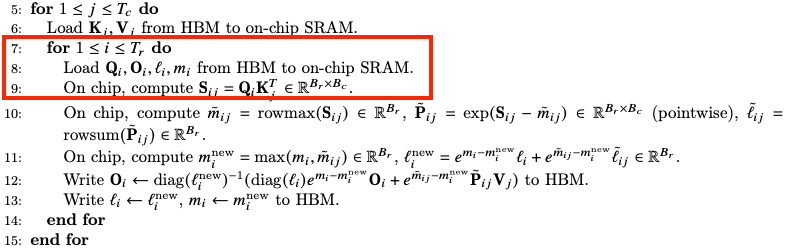
The inner loop visits the $T_r$ query blocks to compute score tiles and, in the subsequent steps, update the output.
First, it loads $Q_i$, $O_i$, $\ell_i$, and $m_i$ from HBM.
It then computes the score tile $S_{ij}$.
I put together the following diagram to make this step easier to picture.
Lines 10–13
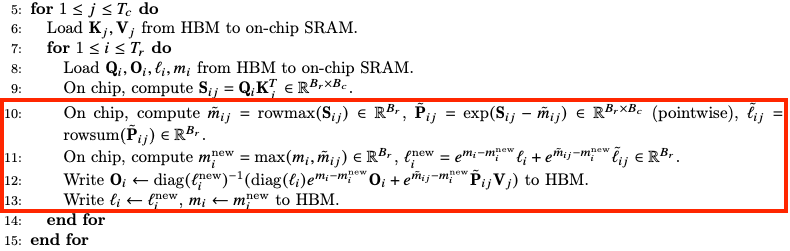
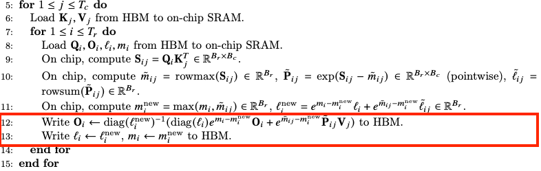
This is where the blockwise softmax calculation and rescaling come together. First, the algorithm computes the maximum of each row in $S_{ij}$, giving $\tilde{m}_{ij}$. It then computes $\tilde{P}_{ij}$ and $\tilde{\ell}_{ij}$, corresponding to the exponentials $f(x)$ and their sum $\ell(x)$ in the softmax formula. At this point, $\tilde{P}_{ij}$ has not yet been normalized into probabilities.
These quantities cover only the current column block $j$. To account for the full row, we need to rescale them. As a quick reminder, this is the identity we are using:
The algorithm updates the running statistics to $m_i^{\mathrm{new}}$ and $\ell_i^{\mathrm{new}}$.
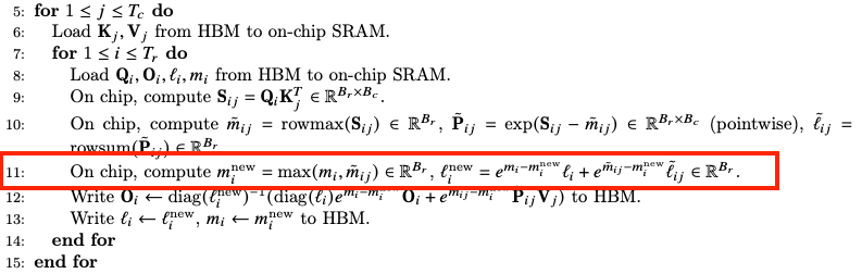
Next, it adjusts the output accumulated so far. The paper combines softmax normalization and the computation of the attention output $O$, rather than treating them as separate stages that materialize the full $P$. This makes the equation look a little complicated, but the idea is fairly simple.
- Undo the normalization of the previous output and rescale it to the new maximum: $\operatorname{diag}(\ell_i)e^{m_i-m_i^{\mathrm{new}}}O_i$.
- Add the contribution from the current block, rescaled to the same reference: $e^{\tilde{m}_{ij}-m_i^{\mathrm{new}}}\tilde{P}_{ij}V_j$.
- Normalize again by dividing by the updated exponential sum: $\operatorname{diag}(\ell_i^{\mathrm{new}})^{-1}$.
The exponential factors above scale rows, following the paper’s notation.
Finally, it writes $O_i$, $\ell_i$, and $m_i$ back to HBM. Alongside the inputs, the state we retain consists of the accumulated output and the small per-row statistics. The intermediate score and exponential tiles are discarded after their contributions have been used. Avoiding full intermediate matrices in HBM is one of the paper’s central contributions.
After all $T_c$ column blocks have been processed, we have the complete attention output $O_i$ for the query row block.
I/O Complexity of FlashAttention
Next, the authors compare the I/O complexity of standard attention with that of FlashAttention.

The appendix works through the derivation in detail. If we break down the nested loops, the outer loop runs $T_c$ times, and each pass through the inner loop visits all of $Q$ and $O$. Both matrices have shape $N \times d$, so the resulting I/O complexity is $\Theta(NdT_c)$. Substituting $T_c = \Theta(Nd/M)$ gives an I/O complexity proportional to $N^2d^2/M$.
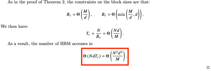
Typical head dimensions $d$ are relatively small, around 64–128, while the available SRAM is on the order of hundreds of kilobytes. We do need to be careful with units here: $M$ in the analysis counts scalar elements, so a capacity in bytes must first be converted using the element size. In the regime where $d^2 < M$, the quadratic term is smaller than in standard attention, whose I/O complexity is $\Theta(Nd + N^2)$.
Block-Sparse FlashAttention
The paper goes a step further with block-sparse FlashAttention, shown in Algorithm 5.
Block-sparse FlashAttention uses a mask matrix $\mathbf{M} \in \{0,1\}^{T_r \times T_c}$, with one entry for each score tile. If $M_{ij}$ is zero, it skips the corresponding tile $S_{ij}$ entirely. This is the condition checked at line 8 of the algorithm.
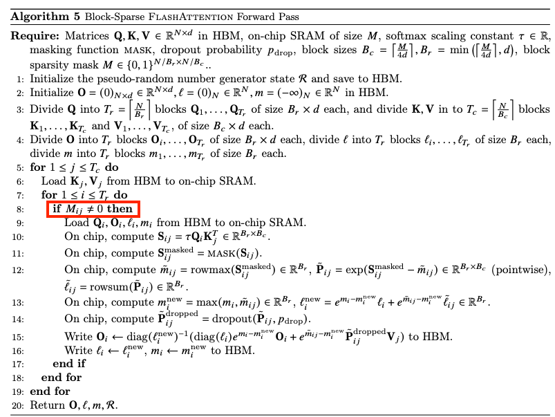
One thing I found surprising was that the choice of which blocks to skip is made in advance. The paper uses a fixed mask based on a butterfly sparsity pattern. The idea of deciding which blocks to leave out before computing any scores felt unfamiliar to me, so I decided to look into it a little more.
Appendix: Sparse Transformer & Pixelated Butterfly
When introducing the butterfly sparsity pattern, the paper directly cites Dao et al.’s Pixelated Butterfly: Simple and Efficient Sparse Training for Neural Network Models (ICLR 2022). Looking through related work also led me to Child et al.’s Sparse Transformer (2019), an early representative work on sparse attention. Since this post is about FlashAttention, I will keep this detour relatively brief.
Sparse Attention
The authors observed some interesting attention patterns in an autoregressive Transformer trained to generate images pixel by pixel. More specifically, they examined the attention learned by a 128-layer self-attention network trained with full attention on CIFAR-10 and highlighted four types of patterns.
- a) In many early layers, attention concentrated on locations near the pixel being generated.
- b) In layers 19 and 20, attention concentrated along horizontal and vertical lines relative to the current pixel.
- c) Some layers showed global, input-dependent patterns that were not confined to nearby locations.
- d) In deeper layers, particularly layers 64–128, attention was highly sparse, with particular locations becoming active only for specific input patterns.
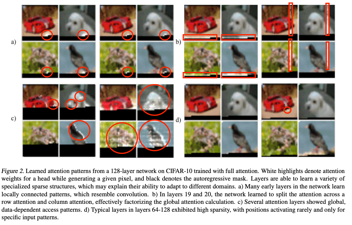
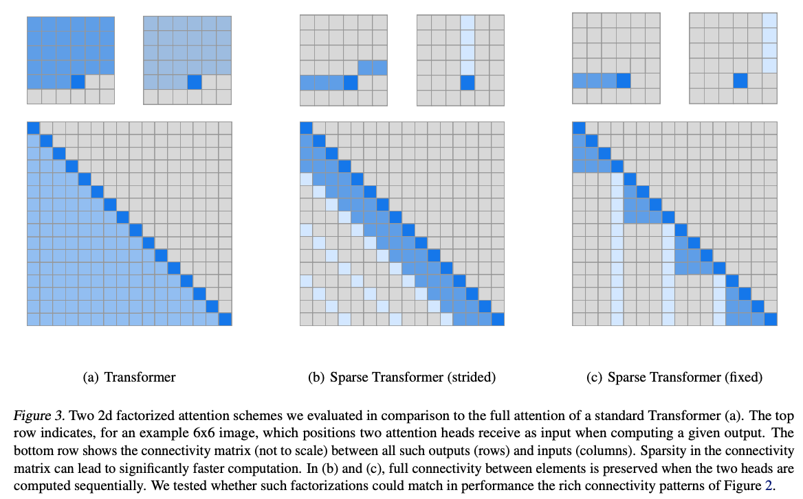
Motivated by these observations, the authors proposed two predefined attention patterns, strided and fixed, and computed attention weights only at the locations allowed by those patterns.
The strided pattern combines attention to nearby locations with attention to locations separated by a regular stride. The paper describes it as a useful fit for data whose structure aligns with that stride, such as images and certain kinds of audio. For text, where relevant relationships do not follow the same regular spacing, it was less effective in their experiments.
For these cases, the authors introduced the fixed pattern. It divides the input into blocks, allows attention within the current block to the current and earlier positions, and makes the last $c$ positions of previous blocks available to later blocks. For example, with a block size of 128 and $c=8$, the final eight positions in each block act as connections to later blocks. In the first block, these are positions 120–127 when counting from zero.
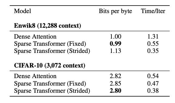
With an appropriate pattern, sparse attention maintained or improved on the modeling performance of dense attention while reducing training time per iteration. On the text benchmark Enwik8, the fixed Sparse Transformer achieved better modeling performance while reducing the reported time per iteration from 1.31 to 0.55. On CIFAR-10, the strided model also improved modeling performance, with time per iteration falling from 0.54 to 0.38.
Pixelated Butterfly
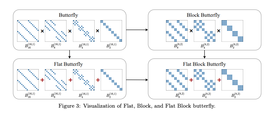
Pixelated Butterfly makes butterfly-based structures more hardware-friendly through block and flat variants. The aim is to use GPUs more efficiently and speed up training across different parts of a network, including attention and MLP layers. Its contributions go beyond an attention pattern, but for this post, I am looking at it as another approach to the broader idea of sparse computation we just discussed.
Experiments
The paper evaluates FlashAttention from several angles, including training speed, perplexity, and benchmark performance.
Faster Models
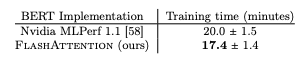
At the time of publication, FlashAttention improved on the existing single-node BERT training record, reducing the time from 20.0 minutes to 17.4 minutes. That is about a 1.15× speedup, or a 13% reduction in elapsed time.
In the GPT-2 experiments on OpenWebText, the authors reported comparable perplexity with substantially shorter training times. For GPT-2 small, FlashAttention was up to 3.5× faster than the Hugging Face implementation and about 1.7× faster than Megatron-LM.

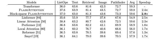
On the Long Range Arena (LRA) benchmark, FlashAttention achieved the highest average accuracy among the compared methods, at 59.8, with a 2.4× speedup. Block-sparse FlashAttention reached an average accuracy of 59.6 and a larger 2.8× speedup.
Better Models with Longer Sequences
The authors also show that better memory efficiency makes it possible to train with longer contexts. In the GPT-2 experiments, they compared context lengths from 1K to 4K. FlashAttention with a 4K context trained faster than the Megatron-LM baseline with a 1K context, despite using four times as much context. The longer context also improved perplexity on OpenWebText from 18.2 to 17.5.
